Description of a network using ring
Ring statistics are mainly used to obtain a snapshot of the connectivity of a network. Thereby the better the snapshot will be, the better the description and the understanding of the properties of the material will be. In the literature many papers present studies of materials using ring statistics. In these studies either the number of Rings per Node '
An example is proposed with a very simple network illustrated in figure 5.19.
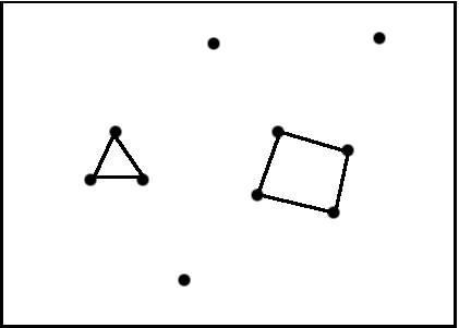
This network is composed of 10 nodes, arbitrary of the same chemical species, and 7 bonds. Furthermore it is clear that in this network there are 1 ring with 3 nodes and 1 ring with 4 nodes.
It is easy to calculate
| 3 | 1/10 |
| 4 | 1/10 |
| 3 | 3/10 |
| 4 | 4/10 |
In the literature the values of
Nevertheless these two properties are not sufficient in order to describe a network using rings. A simple example is proposed in figure 5.20.
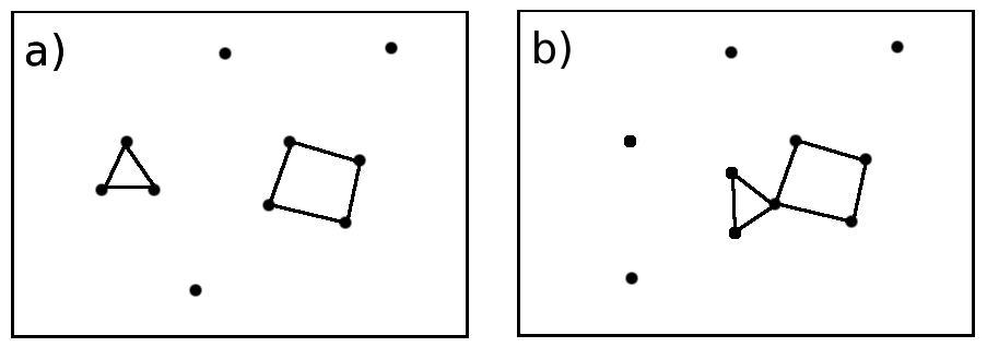
The two networks [Fig. 5.20-a] and [Fig. 5.20-b] do have very similar compositions with 10 nodes and 7 links but they are clearly different. Nevertheless the previous definitions of rings per cell and rings per node even taken together will lead to the same description for these two different networks [Tab. 5.3].
| 3 | 1/10 |
| 4 | 1/10 |
| 3 | 3/10 |
| 4 | 4/10 |
In both cases a) and b) there are 1 ring with 3 nodes and 1 ring with 4 nodes. It has to be noticed that these two rings have properties which correspond to each of the definitions introduced previously (King, Guttman, primitive and strong).
Thus none of these definitions is able to help to distinguish between these two networks. Therefore even though these simple networks are different, the previous definitions lead to the same description.
Thereby it is justified to wonder about the interpretation of the data presented in the literature for amorphous systems with a much higher complexity.
- J. P. Rino, I. Ebbsjö, R. K. Kalia, A. Nakano, and P. Vashishta, Phys. Rev. B., vol. 47, no. 6, pp. 3053–3062, 1993.
- R. M. Van Ginhoven, H. Jónsson, and L. R. Corrales, Phys. Rev. B., vol. 71, no. 2, p. 024208, 2005.
- M. Cobb, D. A. Drabold, and R. L. Cappelletti, Phys. Rev. B., vol. 54, no. 17, pp. 12162–12171, 1996.
- X. Zhang and D. A. Drabold, Phys. Rev. B., vol. 62, no. 23, pp. 15695–15701, 2000.
- D. N. Tafen and D. A. Drabold, Phys. Rev. B., vol. 71, no. 5, p. 054206, 2005.