Rings and connectivity: the R.I.N.G.S. method implemented in Atomes

In the Atomes program the results of the ring statistics analysis are outputted following the new R.I.N.G.S. method [1], [2], this method is presented in the next pages.

The first goal of ring statistics is to give a faithful description of the connectivity of a network and to allow to compare this information with others obtained for already existing structures. It is therefore important to find a guideline which allows to establish a distinction and then a comparison between networks studied using ring statistics. We propose thereafter a new method to achieve this goal. First of all we noticed fundamental points that must be considered to get a reliable and transferable method:

1. The results must be reduced to the total number of nodes in the network.
   The nature of the nodes used to initiate the analysis when looking for rings will have a significant influence, therefore it is essential to reduce the results to a value for one node. Otherwise it would be impossible to compare the results to the ones obtained for systems made of nodes (particles) of different number and/or nature.
   

2. Different networks must be distinguishable whatever the method used to define a ring.
   Indeed it is essential for the result of the analysis to be trustworthy independently of the method used to define a ring (King, Guttman, primitives, strong). Furthermore this will allow to compare the results of these different ring statistics.

Number of rings per cell '\(R_C\)'

We have already introduced this value, which is the first and the easiest way to compare networks using ring statistics.

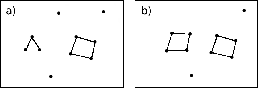
In the most simple cases, such as the one represented in figure 5.21, the networks can be distinguished using only the number of rings [Tab. 5.5]. Nevertheless in most of the cases other information are needed to describe accurately the connectivity of the networks.

Description of the connectivity: difference between rings and nodes

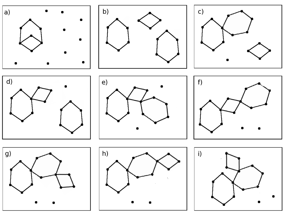
The second information needed to investigate the properties of a network using rings is the evaluation of the connectivity between rings. Indeed the distribution of the ring sizes gives a first information on the connectivity, nevertheless it can not be exactly evaluated unless one studies how the rings are connected. The impact of the relations between rings, already presented in figure 5.20, has been illustrated in detail in figure 5.22. Figure 5.22 represents the different possibilities to combine 2 rings with 6 nodes and 1 ring with 4 nodes in a network composed of 16 nodes.

Among the 9 networks presented in figure 5.22 none can be distinguished using the \(R_C\) value [Tab. 5.7].

Furthermore it is not possible to distinguish these networks using the \(R_N\) value.

It seems possible to isolate the case a) [Tab. 5.8] from the other cases b) \(\to\) i) [Tab. 5.8]. Nevertheless the results obtained using the primitive rings criterion are similar for all cases a) \(\to\) i) [Tab. 5.8], this is in contradiction with the second statement [[Pr2]] proposed in our method.

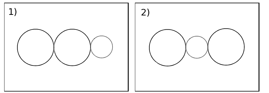
Before introducing parameters able to distinguish the configurations presented in figure 5.22 it is important to wonder about the number of cases to distinguish. From the point of view of the connectivity of the rings, configurations a), b), c) and d) are clearly different. Nevertheless following the same approach configurations e) and f) on the one hand and configurations g), h) and i) on the other hand are identical. A schematic representation [Fig. 5.23] is sufficient to illustrate the similarity of the relations between these networks. The difference between each of these networks does not appear in the connectivity of the rings but in the connectivity of the particles.

Thus among the networks illustrated in figure 5.22 six dispositions of the rings have to be distinguished (a, b, c, d, e, g). The proportions of particles involved, or not involved, in the construction of rings will become an important question.

The new tool defined in our method is able to describe accurately the information still missing on the connectivity. It is a square symmetric matrix of size \((R-r+1)\times (R-r+1)\), where \(R\) and \(r\) represent respectively the bigger and the smaller size of a ring found when analyzing the network: we have called this matrix the connectivity matrix [Tab. 5.9].

The diagonal elements \(P_N(i)\) of this matrix represent the Proportion of Nodes at the origin of at least one ring of size \(i\). And the non-diagonal elements \(P_N(i,j)\) represent the Proportion of Nodes at the origin of ring(s) of size \(i\) and \(j\).
The matrix elements have a value ranging between 0 and 1. The lowest and non equal to 0 is of the form \(\frac{1}{Nn}\), the highest and non equal to 1 is of the form \(\frac{Nn-1}{Nn}\), where \(Nn\) represents the number of nodes in the network.

The connectivity matrix of the configurations illustrated in figure 5.22 are presented in table 5.12. We see that this matrix allows to distinguish each network whatever the way used to define a ring is. This matrix remains simple for small systems (crystalline or amorphous) or when using a small maximum ring size for the analysis. Nevertheless its reading can be considerably altered when analysing amorphous systems with a high maximum ring size for the analysis.

To simplify the reading and the interpretation of the data contained in this matrix for more complex systems, we chose a similar approach to extract information on the connectivity between the rings. As a first step we decided to evaluate only the diagonal elements \(P_N(n)\) of the general connectivity matrix. Indeed these values allow us to obtain a better view of the connectivity than the standard \(R_N\) value.

It is clear [Tab. 5.14] that using \(P_N(n)\) improves the separation between the networks illustrated in figure 5.22. Nevertheless \(P_N(n)\) does not allow to distinguish each of them. We notice that the distinction between networks is improved [Tab. 5.14] in particular when compared to the one obtain with \(R_N(n)\) [Tab. 5.8].

Therefore in a second step we chose to calculate two properties whose definitions are very similar to the one of \(P_N(n)\). The first, named \(P_{N_{\text{max}}}(n)\), represents the proportion of nodes for which the rings with \(n\) nodes are the longest closed paths found using these nodes to initiate the search. The second named, \(P_{N_{\text{min}}}(n)\), represents the proportion of nodes for which the rings with \(n\) nodes are the shortest closed paths found using these nodes to initiate the search.
The terms longest and shortest path must be considered carefully to avoid any confusion with the terms used in section 5.5.2 to define the rings. For one node it is possible to find several rings whose properties correspond to the definitions proposed previously (King's, Guttman's, primitive or strong ring criterion). These rings are solutions found when looking for rings using this particular node to initiate the analysis. In order to calculate \(P_{N_{\text{max}}}(n)\) and \(P_{N_{\text{min}}}(n)\) the longest and the shortest path have to be determined among these different solutions.
\(P_{N_{\text{max}}}(n)\) and \(P_{N_{\text{min}}}(n)\) have values ranging between 0 and \(P_N(n)\). The lowest and non equal to 0 is of the form \(\frac{1}{Nn}\), the highest and non equal to 1 is of the form \(\frac{Nn-1}{Nn}\), where \(Nn\) represents the total number of nodes in the network. For the minimum ring size, \(s_{min}\), existing in the network or found during the search, \(P_{N_{min}}(s_{min})=P_N(s_{min})\). In the same way for the maximum ring size, \(s_{max}\), existing in the network or found during the search, \(P_{N_{max}}(s_{max})=P_N(s_{max})\).

To clarify these information it is possible to normalize \(P_{N_{\text{max}}}(n)\) and \(P_{N_{\text{min}}}(n)\) by \(P_N(n)\). By reducing these values we obtain, for each size of rings, values independent of the total number of nodes \(Nn\) of the system. Then for a considered ring size the values only refer to the number of nodes where the search returns rings of this size: \[P_{max}(n) = \frac{P_{N_{max}}(n)}{P_N(n)} \quad \text{and} \quad P_{min}(n) = \frac{P_{N_{min}}(n)}{P_N(n)} \nonumber\] The normalized terms \(P_{\text{max}}(n)\) and \(P_{\text{min}}(n)\) have values ranging between 0 and 1. The lowest and non equal to 0 is of the form \(\frac{1}{Nn}\), the highest and non equal to 1 is of the form \(\frac{Nn-1}{Nn}\). For the minimum ring size, \(s_{min}\), existing in the network or found during the search, \(P_{min}(s_{min})=1\). In the same way for the maximum ring size, \(s_{max}\), existing in the network or found during the search, \(P_{max}(s_{max})=1\).
\(P_{\text{max}}(n)\) and \(P_{\text{min}}(n)\) give complementary information to the ones obtained with \(R_C(n)\) and \(P_N(n)\) in order to distinguish and compare networks using ring statistics. We can illustrate this result by presenting the complete information obtained with this method [Tab. 5.17] for the networks represented in figure 5.22.

\(P_{\text{max}}(n)\) and \(P_{\text{min}}(n)\) give information about the connectivity of the rings with each other as a function of their size. If a ring of size \(n\) is found using a particular node to initiate the search, \(P_{\text{max}}(n)\) gives the probability that this ring is the longest ring which can be found using this node to initiate the search. At the opposite, \(P_{\text{min}}(n)\) gives the probability that this ring is the shortest ring which can be found using this node to initiate the search.
Thereafter we will use the terms 'connectivity profile' to designate the results of a ring statistics analysis. This profile is related to the definition of rings used in the search and is made of the 4 values defined in our method: \(R_C(n)\), \(P_N(n)\), \(P_{\text{max}}(n)\) and \(P_{\text{min}}(n)\).

The Atomes program provides access to the connectivity profile of the system under study and allows to choose the study the connectivity using all the different methods used to define a ring. Thus King's rings, Guttman's rings, Primitive rings as well as Strong rings analysis are available.

1. S. Le Roux and P. Jund, Comp. Mat. Sci., vol. 49, pp. 70–83, 2010.
2. S. Le Roux and P. Jund, Comp. Mat. Sci., vol. 50, p. 1217, 2011.