Definitions

King's shortest paths criterion

The first way to define a ring has been given by Shirley V. King [1] (and later by Franzblau [2]). In order to study the connectivity of glassy SiO\(_2\) she defines a ring as the shortest path between two of the nearest neighbors of a given node [Fig. 5.13].

King's criterion in the ring statistics: a ring represents the shortest path between two of the nearest neighbors (N1 and N2) of a given node (At).

In the case of the King's criterion one can calculate the maximum number of different ring sizes, \(NS_{max}(KSP)\), which can be found using the atom At to initiate the search: \[\label{lmaxsp} NS_{max}(KSP)\ =\ \frac{Nc({\textbf{At}}) \times (Nc({\textbf{At}})-1)}{2}\] where \(N_c({\textbf{At}})\) is the number of neighbors of atom At. \(NS_{max}(KSP)\) represents the number of ring sizes found if all couples of neighbors of atom At are connected together with paths of different sizes.
It is also possible to calculate the theoretical maximum size, \(TMS(KSP)\), of a King's shortest path ring in the network using: \[\label{tmsking} TMS(KSP)\ = 2\ \times\ (D_{max}\ -\ 2)\ \times (Nc_{max}\ -\ 2)\ +\ 2\ \times\ D_{max}\] where \(D_{max}\) is the longest distance, in number of chemical bonds, separating two atoms in the network, and \(Nc_{max}\) represents the average number of neighbors of the chemical species of higher coordination. If used when looking for rings, periodic boundary conditions have to be taken into account to calculate \(D_{max}\). The relation [Eq. [tmsking]] is illustrated in figure 5.16-2).

Guttman's shortest paths criterion

A later definition of ring was proposed by Guttman [3], who defines a ring as the shortest path which comes back to a given node (or atom) from one of its nearest neighbors [Fig. 5.14].

Guttman's criterion in the ring statistics: a ring represents the shortest path which comes back to a given node (At) from one of its nearest neighbors (N).

Differences between the King and the Guttman's shortest paths criteria are illustrated in figure 5.15.

Differences between the King and the Guttman shortest paths criteria for the ring statistics in an AB_2 system. In these two examples the search is initiated from chemical species A (blue square). The nearest neighbor(s) of chemical species B (green circles) are used to continue the analysis. 1) In the first example only rings with 4 nodes are found using the Guttman's criterion, whereas rings with 18 nodes are also found using the King's criterion (2^9 rings with 18 nodes). 2) In the second example the King's shortest path criterion allows to find the ring with 8 nodes ignored by the Guttman's criterion which is only able to find the rings with 6 nodes.

Like for the King's criterion, with the Guttman's criterion one can calculate the maximum number of different ring sizes, \(NS_{max}(GSP)\), which can be found using the atom At to initiate the search: \[NS_{max}(GSP) = N_c({\textbf{At}}) - 1\] where \(N_c({\textbf{At}})\) is the number of neighbors of atom At. \(NS_{max}(GSP)\) represents the number of ring sizes found if the neighbors of atom At are connected together with paths of different sizes.
It is also possible to calculate the Theoretical Maximum Size, \(TMS(GSP)\), of a Guttman's ring in the network using: \[\label{tmsg} TMS(GSP)\ = 2\ \times\ D_{max}\] where \(D_{max}\) represents the longest distance, in number of chemical bonds, separating two atoms in the network. If used when looking for rings, periodic boundary conditions have to be taken into account to calculate \(D_{max}\). The relation [Eq. [tmsg]] is illustrated in figure 5.16-1.

Theoretical maximum size of the rings for an AB_2 system (Nc_{max}~=~Nc_{A}~=~4) and using: 1) the Guttman's criterion, 2) the King's criterion. The theoretical maximum size represent the longest distance between two nearest neighbors 1 and 2 (green circles) of the atom At used to initiate the search (blue square).

Since the introduction of the King's and the Guttman's criteria other definitions of rings have been proposed. These definitions are based on the properties of the rings to be decomposed into the sum of smaller rings.

The primitive rings criterion

A ring is primitive [4], [5] (or Irreducible [6]) if it can not be decomposed into two smaller rings [Fig. 5.17].

Primitive rings in the ring statistics: the 'AC' ring defined by the sum of the A and the C paths is primitive only if there is no B path shorter than A and shorter than C which allows to decompose the 'AC' ring into two smaller rings 'AB' and 'AC'.

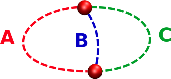
The primitive rings analysis between the paths in figure 5.17 may lead to 3 results depending on the relations between the paths A, B, and C:

  • If paths A, B, and C have the same length: A = B = C then the rings 'AB', 'AC' and 'BC' are primitives.

  • If the relation between the paths is like \(?=?<?\) (ex: A = B < C) then 1 smaller ring ('AB') and 2 bigger rings ('AC' and 'BC') exist. None of these rings can be decomposed into the sum of two smaller rings therefore the 3 rings are again primitives.

  • If the relation between the path is like \(?<?=?\) (ex: A < B = C) or \(?<?<?\) (ex: A < B < C) then a shortest path exists (A). It will be possible to decompose the ring ('BC') built without this shortest path into the sum of 2 smaller rings ('AB' and 'AC'), therefore this ring will not be primitive.

The strong rings criterion

The strong rings [4], [5] are defined by extending the definition of primitive rings. A ring is strong if it can not be decomposed into a sum of smaller rings whatever this sum is, ie. whatever the number of paths in the decomposition is.

Strong rings in the ring statistics: a) the 9-carbon-atoms ring created after breaking a C-C bond in a Buckminster fulleren molecule is a counterexample of strong ring; b) the combination of shortest rings, 11 5-carbon-atoms rings and 19 6-carbon-atoms rings, appears easily after the deformation of the C_{60} molecule.

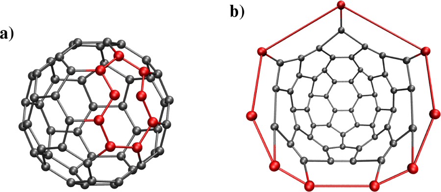
By definition the strong rings are also primitives, therefore to search for strong rings can be summed as to find the strong rings among the primitive rings. This technique is limited to relatively simple cases, like crystals or structures such as the one illustrated in figure 5.18. On the one hand the CPU time needed to complete such an analysis for amorphous systems is very important. On the other hand it is not possible to search for strong rings using the same search depth than for other types of rings. The strong ring analysis is indeed diverging which makes it very complex to implement for amorphous materials.
In the case of primitive rings like in the case of strong rings, there is no theoretical maximum size of rings in the network.

  1. S. V. King, Nat., vol. 213, p. 1112, 1967.
  2. D. S. Franzblau, Phys. Rev. B., vol. 44, no. 10, pp. 4925–4930, 1991.
  3. L. Guttman, J. Non-Cryst. Solids, vol. 116, pp. 145–147, 1990.
  4. K. Goetzke and H. J. Klein, J. Non-Cryst. Solids, vol. 127, pp. 215–220, 1991.
  5. X. Yuan and A. N. Cormack, Comp. Mat. Sci., vol. 24, pp. 343–360, 2002.
  6. F. Wooten, Act. Cryst. A, vol. 58, no. 4, pp. 346–351, 2002.