Partial structure factors

There are a few, somewhat different definitions of partials \(S(q)\) used in practice, and computed by Atomes

Faber-Ziman definition/formalism

One way used to define the partial structure factors has been proposed by Faber and Ziman [1]. In this approach the structure factor is represented by the correlations between the different chemical species. To describe the correlation between the \(\alpha\) and the \(\beta\) chemical species the partial structure factor \(S^{FZ}_{\alpha \beta}(q)\) is defined by: \[\label{sqp0} S^{FZ}_{\alpha \beta}(q)\ =\ 1\ +\ 4 \pi \rho \int_{0}^{\infty}\ dr\ r^{2}\ \frac{\sin qr}{qr}\ \left(g_{\alpha \beta}(r)-1\right)\] where the \(g_{\alpha \beta}(r)\) are the partial radial distribution functions [Eq. [g2r_4]].
The total structure factor is then obtained by the relation: \[\label{sqp1} S(q)\ =\ \sum_{\alpha,\beta}\ c_{\alpha} b_{\alpha}\ c_{\beta} b_{\beta}\ \left[S^{FZ}_{\alpha \beta}(q)\ -\ 1\right]\]

Ashcroft-Langreth definition/formalism

In a similar approach, based on the correlation between the chemical species, and developed by Ashcroft and Langreth [2], [3], [4], the partial structure factors \(S^{AL}_{\alpha \beta}(q)\) are defined by: \[\label{sqp2} S^{AL}_{\alpha \beta}(q)\ =\ \delta_{\alpha \beta}\ +\ 4 \pi \rho \left({c_\alpha c_\beta}\right)^{1/2}\ \int_{0}^{\infty}\ dr\ r^{2}\ \frac{\sin qr}{qr}\ \left(g_{\alpha \beta}(r)-1\right)\] where \(\delta_{\alpha \beta}\) is the Kronecker delta, \(c_\alpha = \displaystyle{\frac{N_\alpha}{N}}\), and the \(g_{\alpha \beta}(r)\) are the partial radial distribution functions [Eq. [g2r_4]].
Then the total structure factor can be calculated using: \[\label{sqp3} S(q)\ =\ \frac{\displaystyle{\sum_{\alpha, \beta}}\ b_\alpha b_\beta\ \left({c_\alpha c_\beta}\right)^{1/2}\ \left[S^{AL}_{\alpha \beta}(q)\ +\ 1\right]}{\displaystyle\sum_{\alpha}\ c_\alpha b_\alpha^2}\]

Bhatia-Thornton definition/formalism

In this approach, used in the case of binary systems AB\(_x\) [5] only, the total structure factor \(S(q)\) can be express as the weighted sum of 3 partial structure factors: \[\label{sqp4} S(q)= \frac{\langle b \rangle^2 S_{NN}(q) + 2\langle b \rangle(b_\text{A} -b_\text{B})S_{NC}(q) + (b_\text{A}-b_\text{B})^2S_{CC}(q) - (c_\text{A} b_\text{A}^2 + c_\text{B} b_\text{B}^2)}{\langle b \rangle^2}\ +\ 1\] where \(\langle b \rangle = c_\text{A} b_\text{A} + c_\text{B} b_\text{B}\), with \(c_\text{A}\) and \(b_\text{A}\) representing respectively the concentration and the scattering length of species \(\text{A}\).
\(S_{NN}(q)\), \(S_{NC}(q)\) and \(S_{CC}(q)\) represent combinations of the partial structure factors calculated using the Faber-Ziman formalism and weighted using the concentrations of the 2 chemical species: \[\label{sqp5} S_{NN}(q) = \sum_{\text{A}=1}^{2} \sum_{\text{B}=1}^{2} c_{\text{A}} c_{\text{B}} S^{FZ}_{\text{A} \text{B}}(q)\] \[\label{sqp6} S_{NC}(q) = c_{\text{A}} c_{\text{B}} \times \left[\ c_\text{A}\times\left(S^{FZ}_{\text{A}\text{A}}(q) - S^{FZ}_{\text{A} \text{B}}(q)\right)\ -\ c_{\text{B}}\times\left(S^{FZ}_{\text{B}\text{B}}(q) - S^{FZ}_{\text{A} \text{B}}(q)\right)\ \right]\] \[\label{sqp7} S_{CC}(q) = c_{\text{A}} c_{\text{B}} \times \left[ 1 + c_{\text{A}} c_{\text{B}} \times \left[ \sum_{\text{A}=1}^{2} \sum_{\text{B}\ne\text{A}}^{2} \left( S^{FZ}_{\text{A}\text{A}}(q) - S^{FZ}_{\text{A}\text{B}}(q) \right)\right] \right]\]

\(\bullet\)

\(S_{NN}(q)\) is the Number-Number partial structure factor.
Its Fourier transform allows to obtain a global description of the structure of the solid, ie. of the distribution of the experimental scattering centers, or atomic nuclei, positions. The nature of the chemical species spread in the scattering centers is not considered. Furthermore if \(b_\text{A} =b_\text{B}\) then \(S_{NN}(q) = S(q)\).

\(\bullet\)

\(S_{CC}(q)\) is the Concentration-Concentration partial structure factor.
Its Fourier transform allows to obtain an idea of the distribution of the chemical species over the scattering centers described using the \(S_{NN}(q)\). Therefore the \(S_{CC}(q)\) describes the chemical order in the material. In the case of an ideal binary mixture of 2 chemical species \(A\) and \(B\)2, \(S_{CC}(q)\) is constant and equal to \(c_Ac_B\). In the case of an ordered chemical mixture (chemical species with distinct diameters, and with heteropolar and homopolar chemical bonds) it is possible to link the variations of the \(S_{CC}(q)\) to the product of the concentrations of the 2 chemical species of the mixture:

  • \(S_{CC}(q) = c_Ac_B\): random distribution.

  • \(S_{CC}(q) > c_Ac_B\): homopolar atomic correlations (A-A, B-B) preferred.

  • \(S_{CC}(q) < c_Ac_B\): heteropolar atomic correlations (A-B) preferred.

  • \(\langle b \rangle = 0\): \(S_{CC}(q) = S(q)\).

\(\bullet\)

\(S_{NC}(q)\) is the Number-Concentration partial structure factor.
Its Fourier transform allows to obtain a correlation between the scattering centers and their occupation by a given chemical species. The more the chemical species related partial structure factors are different (\(S_{AA}(q) \ne S_{BB}(q)\)) and the more the oscillations are important in the \(S_{NC}(q)\). In the case of an ideal mixture \(S_{NC}(q) = 0\), and all the information about the structure of the system is given by the \(S_{NN}(q)\).

If we consider the binary mixture as an ionic mixture then it is possible to calculate the Charge-Charge \(S_{ZZ}(q)\) and the Number-Charge \(S_{NZ}(q)\) partial structure factors using the Concentration-Concentration \(S_{CC}(q)\) and the Number-Concentration \(S_{NC}(q)\): \[\label{sqp8} S_{ZZ}(q) = \frac{S_{CC}(q)}{c_A c_B} \qquad and \qquad S_{NZ}(q) = \frac{S_{NC}(q)}{c_B/Z_A}\] \(c_A\) and \(Z_A\) represent the concentration and the charge of the chemical species A, the global neutrality of the system must be respected therefore \(c_AZ_A + c_BZ_B=0\).

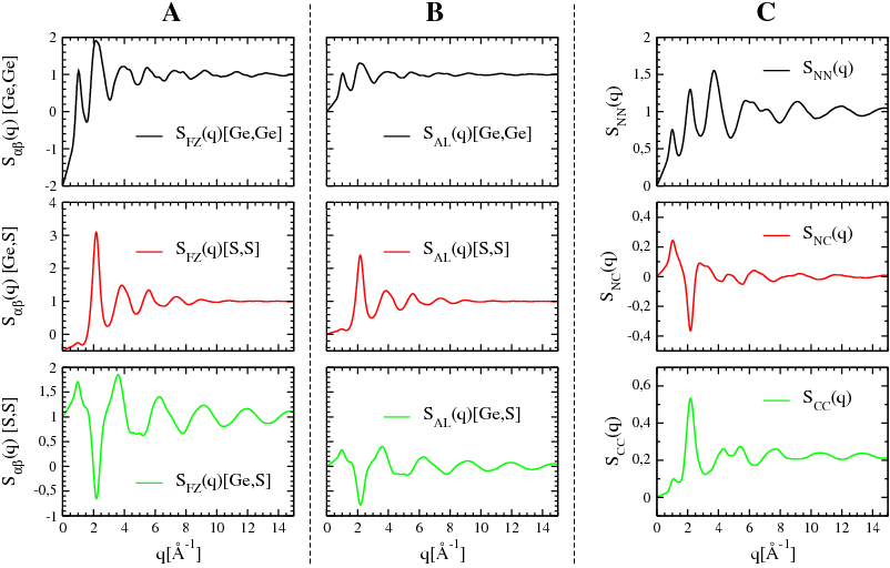
Figure 5.6 illustrates, and allows to compare, the partial structure factors of glassy GeS\(_2\) at 300 K calculated in the different formalism Faber-Ziman [1], Ashcroft-Langreth [2], [3], [4], and Bhatia-Thornton [5].

Partial structure factors of glassy GeS_2 at 300 K. A Faber-Ziman , B Ashcroft-Langreth and C Bhatia-Thornton .

  1. Particles that can be described using spheres of the same diameter and occupying the same molar volume, subject to the same thermal constrains, in a mixture where the substitution energy of a particle by another is equal to zero.↩︎

  1. T. E. Faber and Z. J. M., Phil. Mag., vol. 11, no. 109, pp. 153–173, 1965.
  2. N. W. Ashcroft and D. C. Langreth, Phys. Rev., vol. 156, no. 3, pp. 685–692, 1967.
  3. N. W. Ashcroft and D. C. Langreth, Phys. Rev., vol. 159, no. 3, pp. 500–510, 1967.
  4. N. W. Ashcroft and D. C. Langreth, Phys. Rev., vol. 166, no. 3, p. 934, 1968.
  5. A. B. Bhatia and D. E. Thornton, Phys. Rev. B., vol. 2, no. 8, pp. 3004–3012, 1970.